Image similarity estimation using a Siamese Network with a contrastive loss

Introduction

Siamese Networks are neural networks which share weights between two or more sister networks, each producing embedding vectors of its respective inputs.

In supervised similarity learning, the networks are then trained to maximize the contrast (distance) between embeddings of inputs of different classes, while minimizing the distance between embeddings of similar classes, resulting in embedding spaces that reflect the class segmentation of the training inputs.

Setup

library(keras3)

Hyperparameters

epochs <- 10
batch_size <- 16
margin <- 1  # Margin for contrastive loss.

Load the MNIST dataset

c(c(x_train_val, y_train_val), c(x_test, y_test)) %<-% dataset_mnist()

Define training and validation sets

# Keep 50% of the training data in the validation set.
train_indices <- seq_len(30000L)
validation_indices <- seq.int(30001L, nrow(x_train_val))

x_train <- x_train_val[train_indices, , , drop = FALSE]
x_val <- x_train_val[validation_indices, , , drop = FALSE]
y_train <- y_train_val[train_indices]
y_val <- y_train_val[validation_indices]
rm(x_train_val, y_train_val)

# Change the data type to a floating point format and make the channel
# dimension explicit.
as_image_tensor <- function(x) {
  x |>
    op_convert_to_tensor(dtype = "float32") |>
    op_expand_dims(axis = -1)
}

x_train <- as_image_tensor(x_train)
x_val <- as_image_tensor(x_val)
x_test <- as_image_tensor(x_test)

Create pairs of images

We will train the model to differentiate between digits of different classes. For example, digit 0 needs to be differentiated from the rest of the digits (1 through 9), digit 1 from 0 and 2 through 9, and so on. To carry this out, we select N random images from class A (for example, digit 0) and pair them with N random images from another class B (for example, digit 1). We repeat this process for all classes of digits.

make_pairs <- function(x, y) {
  num_classes <- max(y) + 1L
  digit_indices <- lapply(
    seq_len(num_classes) - 1L,
    \(label) which(y == label)
  )

  matching_indices <- vapply(
    seq_along(y),
    \(i) sample(digit_indices[[y[[i]] + 1L]], size = 1L),
    integer(1)
  )

  nonmatching_labels <- vapply(
    y,
    \(label) {
      candidates <- setdiff(seq_len(num_classes) - 1L, label)
      as.integer(sample(candidates, size = 1L))
    },
    integer(1)
  )
  nonmatching_indices <- vapply(
    seq_along(y),
    \(i) {
      sample(digit_indices[[nonmatching_labels[[i]] + 1L]], size = 1L)
    },
    integer(1)
  )

  first_indices <- rep(seq_along(y), each = 2L)
  second_indices <- as.vector(rbind(matching_indices, nonmatching_indices))

  list(
    pair1 = op_take(x, first_indices, axis = 1),
    pair2 = op_take(x, second_indices, axis = 1),
    labels = as.numeric(rep(c(0, 1), times = length(y)))
  )
}

pairs_train <- make_pairs(x_train, y_train)
pairs_val <- make_pairs(x_val, y_val)
pairs_test <- make_pairs(x_test, y_test)

rm(x_train, x_val, x_test, y_train, y_val, y_test)

We get 60,000 training pairs. Each pair contains two images, and each image has shape (28, 28, 1).

dim(pairs_train$pair1)

## [1] 60000    28    28     1

Split the training pairs:

x_train_1 <- pairs_train$pair1
x_train_2 <- pairs_train$pair2
labels_train <- pairs_train$labels

Split the validation pairs:

x_val_1 <- pairs_val$pair1
x_val_2 <- pairs_val$pair2
labels_val <- pairs_val$labels

Split the test pairs:

x_test_1 <- pairs_test$pair1
x_test_2 <- pairs_test$pair2
labels_test <- pairs_test$labels

Visualize pairs and their labels

visualize <- function(pairs, labels, to_show = 6L, num_col = 3L,
                      predictions = NULL, test = FALSE) {
  num_row <- max(to_show %/% num_col, 1L)
  to_show <- num_row * num_col
  indices <- seq_len(to_show)

  pair1 <- op_take(pairs$pair1, indices, axis = 1) |> as.array()
  pair2 <- op_take(pairs$pair2, indices, axis = 1) |> as.array()
  prediction_values <- if (is.null(predictions)) {
    NULL
  } else {
    drop(as.array(predictions))[indices]
  }

  old_par <- par(no.readonly = TRUE)
  on.exit(par(old_par), add = TRUE)
  par(mfrow = c(num_row, num_col), mar = c(0, 0, 2, 0))

  for (i in indices) {
    image <- cbind(pair1[i, , , 1L], pair2[i, , , 1L])
    plot(as.raster(image / 255))

    label <- if (test) {
      sprintf(
        "True: %d | Pred: %.5f",
        as.integer(labels[[i]]),
        prediction_values[[i]]
      )
    } else {
      sprintf("Label: %d", as.integer(labels[[i]]))
    }
    title(main = label)
  }

  invisible(NULL)
}

Inspect training pairs:

visualize(pairs_train, labels_train, to_show = 4L, num_col = 4L)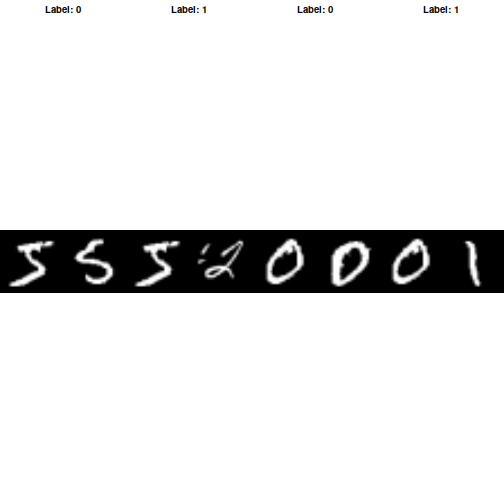

plot of chunk unnamed-chunk-10

Inspect validation pairs:

visualize(pairs_val, labels_val, to_show = 4L, num_col = 4L)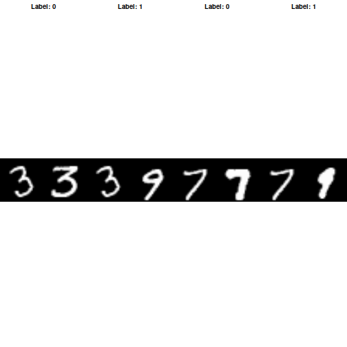

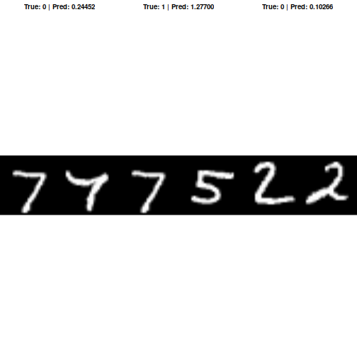
plot of chunk unnamed-chunk-11

Inspect test pairs:

visualize(pairs_test, labels_test, to_show = 4L, num_col = 4L)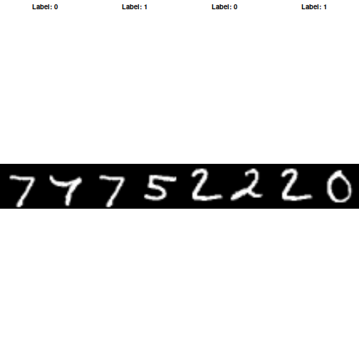

plot of chunk unnamed-chunk-12

Define the model

There are two input layers, each leading to its own network, which produces embeddings. A Lambda layer then merges them using Euclidean distance.

euclidean_distance <- function(vectors) {
  c(x, y) %<-% vectors
  sum_square <- op_sum(op_square(x - y), axis = 2, keepdims = TRUE)
  op_sqrt(op_maximum(sum_square, config_epsilon()))
}

create_embedding_network <- function() {
  inputs <- keras_input(shape = c(28, 28, 1))
  outputs <- inputs |>
    layer_batch_normalization() |>
    layer_conv_2d(
      filters = 4, kernel_size = c(5, 5), activation = "tanh"
    ) |>
    layer_average_pooling_2d(pool_size = c(2, 2)) |>
    layer_conv_2d(
      filters = 16, kernel_size = c(5, 5), activation = "tanh"
    ) |>
    layer_average_pooling_2d(pool_size = c(2, 2)) |>
    layer_flatten() |>
    layer_batch_normalization() |>
    layer_dense(units = 10, activation = "tanh")

  keras_model(inputs, outputs, name = "embedding")
}

embedding_network <- create_embedding_network()

input_1 <- keras_input(shape = c(28, 28, 1))
input_2 <- keras_input(shape = c(28, 28, 1))

# Reusing the same embedding network shares its weights between the towers.
tower_1 <- embedding_network(input_1)
tower_2 <- embedding_network(input_2)

# Distance is the output; there is no final dense sigmoid layer.
distance <- list(tower_1, tower_2) |>
  layer_lambda(euclidean_distance)
siamese <- keras_model(
  inputs = list(input_1, input_2),
  outputs = distance
)

Define the contrastive loss

contrastive_loss <- function(margin = 1) {
  function(y_true, y_pred) {
    square_pred <- op_square(y_pred)
    margin_square <- op_square(op_maximum(margin - y_pred, 0))
    op_mean(
      (1 - y_true) * square_pred +
        y_true * margin_square
    )
  }
}

Define the accuracy metric

accuracy <- function(y_true, y_pred) {
  y_true <- op_cast(y_true, "float32")
  y_true <- op_reshape(y_true, c(-1))
  y_pred <- op_reshape(y_pred, c(-1))

  # 0 for similar (< 0.5), 1 for dissimilar (> 0.5).
  predictions <- op_cast(y_pred > 0.5, "float32")
  op_mean(op_equal(y_true, predictions))
}

Compile the model with the contrastive loss

siamese |> compile(
  loss = contrastive_loss(margin),
  optimizer = "rmsprop",
  metrics = list(accuracy)
)
summary(siamese)

## Model: "functional"
## ┏━━━━━━━━━━━━━━━━━━━┳━━━━━━━━━━━━━━━━━┳━━━━━━━━━━━┳━━━━━━━━━━━━━━━━┳━━━━━━━┓
## ┃ Layer (type)      ┃ Output Shape    ┃   Param # ┃ Connected to   ┃ Trai… ┃
## ┡━━━━━━━━━━━━━━━━━━━╇━━━━━━━━━━━━━━━━━╇━━━━━━━━━━━╇━━━━━━━━━━━━━━━━╇━━━━━━━┩
## │ input_layer_1     │ (None, 28, 28,  │         0 │ -              │   -   │
## │ (InputLayer)      │ 1)              │           │                │       │
## ├───────────────────┼─────────────────┼───────────┼────────────────┼───────┤
## │ input_layer_2     │ (None, 28, 28,  │         0 │ -              │   -   │
## │ (InputLayer)      │ 1)              │           │                │       │
## ├───────────────────┼─────────────────┼───────────┼────────────────┼───────┤
## │ embedding         │ (None, 10)      │     5,318 │ input_layer_1… │   Y   │
## │ (Functional)      │                 │           │ input_layer_2… │       │
## ├───────────────────┼─────────────────┼───────────┼────────────────┼───────┤
## │ lambda (Lambda)   │ (None, 1)       │         0 │ embedding[0][… │   -   │
## │                   │                 │           │ embedding[1][… │       │
## └───────────────────┴─────────────────┴───────────┴────────────────┴───────┘
##  Total params: 5,318 (20.77 KB)
##  Trainable params: 4,804 (18.77 KB)
##  Non-trainable params: 514 (2.01 KB)

Train the model

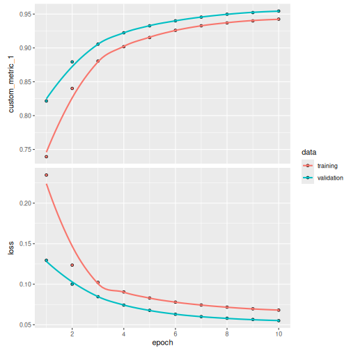
history <- siamese |> fit(
  x = list(x_train_1, x_train_2),
  y = labels_train,
  validation_data = list(
    list(x_val_1, x_val_2),
    labels_val
  ),
  batch_size = batch_size,
  epochs = epochs
)

## Epoch 1/10
## 3750/3750 - 13s - 3ms/step - custom_metric_1: 0.7394 - loss: 0.2346 - val_custom_metric_1: 0.8216 - val_loss: 0.1294
## Epoch 2/10
## 3750/3750 - 9s - 2ms/step - custom_metric_1: 0.8402 - loss: 0.1235 - val_custom_metric_1: 0.8794 - val_loss: 0.1000
## Epoch 3/10
## 3750/3750 - 9s - 2ms/step - custom_metric_1: 0.8806 - loss: 0.1022 - val_custom_metric_1: 0.9056 - val_loss: 0.0846
## Epoch 4/10
## 3750/3750 - 10s - 3ms/step - custom_metric_1: 0.9019 - loss: 0.0904 - val_custom_metric_1: 0.9224 - val_loss: 0.0742
## Epoch 5/10
## 3750/3750 - 10s - 3ms/step - custom_metric_1: 0.9154 - loss: 0.0829 - val_custom_metric_1: 0.9327 - val_loss: 0.0678
## Epoch 6/10
## 3750/3750 - 9s - 2ms/step - custom_metric_1: 0.9260 - loss: 0.0779 - val_custom_metric_1: 0.9400 - val_loss: 0.0629
## Epoch 7/10
## 3750/3750 - 9s - 3ms/step - custom_metric_1: 0.9327 - loss: 0.0743 - val_custom_metric_1: 0.9455 - val_loss: 0.0599
## Epoch 8/10
## 3750/3750 - 9s - 2ms/step - custom_metric_1: 0.9369 - loss: 0.0717 - val_custom_metric_1: 0.9498 - val_loss: 0.0580
## Epoch 9/10
## 3750/3750 - 9s - 3ms/step - custom_metric_1: 0.9400 - loss: 0.0696 - val_custom_metric_1: 0.9522 - val_loss: 0.0564
## Epoch 10/10
## 3750/3750 - 9s - 2ms/step - custom_metric_1: 0.9425 - loss: 0.0680 - val_custom_metric_1: 0.9544 - val_loss: 0.0551

Visualize results

plot(history)

plot of chunk unnamed-chunk-18

Evaluate the model

results <- siamese |> evaluate(
  list(x_test_1, x_test_2),
  labels_test
)

## 625/625 - 1s - 2ms/step - custom_metric_1: 0.9552 - loss: 0.0521

results

## $custom_metric_1
## [1] 0.95515
##
## $loss
## [1] 0.05209473

Visualize the predictions

predictions <- siamese |> predict(list(x_test_1, x_test_2))

## 625/625 - 1s - 2ms/step

visualize(
  pairs_test,
  labels_test,
  to_show = 3L,
  predictions = predictions,
  test = TRUE
)

plot of chunk unnamed-chunk-20